The Color Math Concept
by Ken Davies
The human eye is able to decipher patterns of light according to the
primary colors of the additive system: red, green and blue (RGB). However, it is the
subtractive system’s primaries: cyan, magenta and yellow (CMY) that best lend
themselves to understanding the COLORCUBE and the concept of Color Math. This chapter
unveils the inner workings of the COLORCUBE Model and the tools that are required for
navigation in and about it.
Within any given subtractive color space, as defined by the three primaries CMY, the
use of Color Math will allow us to map the relationships of all the colors encompassed by
that cubic area. Bridging the additive and subtractive systems of color, mixing colors,
selecting color complements and converting color media equivalents all become matters of
mathematics rather than that of guess work or compromise.
Following a brief introduction to basic logic and scientific fundamentals, as they are
relevant to color, we will expand upon the Color Math concept. By the conclusion of this
chapter, we will be able to apply Color Math to a variety of tasks such as dissecting the
COLORCUBE, dispelling critical aspects of traditional color theory, mixing colors,
determining color complements and charting print-to-paint media conversions.
|
| Principles of Color Math The similarity to
commonly applied basics in mathematics and algebra will make these initial color
principles appear somewhat elementary. However, their value will become apparent as the
problems that we will encounter become increasingly complex.
The diagram below illustrates the principle of symmetry that states that the
order in which colors are added to one another does not alter the outcome.
|
Figure 1. Color A + Color B = Color B + Color A |
|
 |
The addition (or subtraction) of two or more colors will likely cause a visible change
in hue but we must also pay particular attention to the cumulative volume of the
operation. For example, mixing one measurable unit of color with another yields twice the
volume of the resulting color. The following diagram highlights this change in quantity
using simple, like colors.
|
Figure 2(a). 1 part Color A + 1 part Color A = 2 parts Color A |
|
 |
Also, this principle of cumulative volume applies to those operations involving
varying colors as well.
|
Figure 2(b). 1 Color A + 1 Color B = 2 Color C |
|
 |
As easy as these fundamentals are to grasp, the visual aids accompanying the upcoming
problems shown may be counter-intuitive. The derivations of the Color Math "building
blocks" presented in the next section will be the first step in making them fully
comprehensible.
|
| Primary Colors We have stated that all of the
colors captured within a color space are functions of the primaries cyan, magenta and
yellow. The vertices or corner points on a COLORCUBE are these three pure hues (labeled A,
B and C below), along with their various combinations. Together, these eight colors
represent the key elements used in all Color Math calculations.
|
Figure 3. Primary colors in the subtractive system |
|
 |
Although considered primary in the additive system of color, red, green and blue are
the secondary colors in the subtractive system. By combining cyan with magenta, cyan with
yellow and magenta with yellow, we are able to make blue, green and red respectively. As
long as each primary ingredient is at full saturation and in equivalent quantities, the
following operations hold true.
|
Figure 4(a). 1 Cyan + 1 Magenta = 2 Blue |
|
 |
|
|
|
Figure 4(b). 1 Cyan + 1 Yellow = 2 Green |
|
 |
|
|
|
Figure 4(c). 1 Magenta + 1 Yellow = 2 Red |
|
 |
When all three primaries are mixed together in equal proportion, the resulting color is
black. (editor’s note: this color mixture is mainly theoretical as we have yet to
encounter perfect subtractive primaries that make a perfect black when mixed.)
|
Figure 5. 1 Cyan + 1 Magenta + 1 Yellow = 3 Black |
|
 |
Black is also achieved when certain combinations of the primary and secondary elements
are mixed. We recall from figure 4 (c), that red is made up of equal parts magenta and
yellow. Therefore, we can add cyan to red in order to form black by virtue of the equation
below:
|
Figure 6. Color A + SUM Colors BC = Color ABC |
|
 |
And so,
|
Figure 7(a). 1 part Cyan + 2 parts Red = 3 parts Black |
|
 |
Because each secondary color is merely a combination of two primaries, black is the
result in each of the following mixtures. Please note the unequal quantities of the inputs
and the constant amount of the sum.
|
Figure 7(b). 1 Magenta + 2 Green = 3 Black |
|
 |
|
|
|
Figure 7(c). 1 Yellow + 2 Blue = 3 Black |
|
 |
The operations shown above may beg the question: what happens when the secondary colors
are added together in equal quantities, as in the diagram below?
|
Figure 8. Red + Green + Blue? |
|
 |
Answering this question correctly requires a break down of each of the inputs into
its’ constituent CMY elements in order to investigate the exact quantities being
mixed. In order to simplify this task, we will take single units of red, green and blue
and discover that they yield the following:
|
Figure 9. Adding Red + Green + Blue (in terms of CMY) |
|
 |
Upon analyzing the CMY proportions in the sum, we recognize the color as black! This
solution may strike you as odd. After all, if equal quantities of primary colors cyan,
magenta and yellow make black, how can the same amounts of secondary colors red, green and
blue possibly produce an identical result? Can the following diagram really be true?
|
Figure 10. 1 Red + 1 Green + 1 Blue = 3 Black |
|
 |
The answer is "yes" because we have learned that, by definition; black is CMY
in equal amounts at full saturation. (If the saturation or purity of the primary hues is
less than full, some form of gray will emerge from the mixture. The value of the gray will
depend on the amount of base color present.) So, in deconstructing red, green and blue
into their respective CMY elements, we discover that these three colors cumulatively do
indeed carry the correct CMY proportions to create black. Color Math will be used later in
the chapter to prove the validity of this conclusion.
|
| White as "Base" Color In the parentheses
above, we alluded briefly to the concept of the base color. This is the color that is
perceived when no primary hues are present. For instance, in color media that utilize the
additive system of color, black is considered to be the base color. That is, the eye
responds to the absence of red, green and blue (primaries in the additive system) and its
perception is the color black. The opposite occurs in the subtractive system where zero
values of cyan, magenta and yellow result in the perception of white.
While the use of a non-white, non-black base is possible; the result is a truncated
colorspace and a somewhat skewed COLORCUBE. Such is the case when looking through tinted
eyewear or offset printing onto colored paper. Thus, in order to maximize the set of
visible colors within our CMY color space, white will be the assumed base color.
To this point in our discussion, all of the colors have been fully saturated containing
no white or base color. We now attempt to understand the impact of the base color by
infusing white base with increasing amounts of primary hues and observe the changes to the
resulting color.
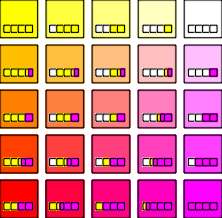
Our analysis begins with total white base to which we add rising increments of yellow
primary. As long as the overall volume of each color sample is held constant, the
progression from 100% white leads to a fully saturated yellow. As the horizontal bars in
the top left diagram show, the reduction of base color, white gives way to an increase of
non-base content. The changes in the "base-to-primary" ratio results in
graduated versions of a mixed color (known as tints due to the presence of white) as shown
in the color circles. The upper right corner of the diagram below maps the same procedure
using magenta primary.
|
Figure 11. Adding primaries to a white base. |
|
 |
Let us now conduct a similar operation with two primary colors adding them both to the
base color, white. We should recognize that the combination of equal parts yellow and
magenta creates red but as illustrated above in the bottom left box, this mixture does not
affect the proportion of the white base. The base color maintains its percentage value of
100, 75, 50, 25 and 0% of the total color respectively, regardless of the amounts of
multiple primaries which make up the remainder.
The same effect takes place when all three primaries are added to decreasing amounts of
white base. As demonstrated in the bottom right corner above, grays and black are the
result of mixing cyan, magenta and yellow with a white base. It is important to remember
from these exercises that the CMY primary mixture occupies only the portion of the color
that is non-base.
|
| Constructing the COLORCUBE Returning momentarily
to the progressions of magenta and yellow tints, we in fact derived two axes of the
COLORCUBE. The plane of color, constructed in the figure 12, is what bridges the color
space that exists between those two axes. Using a similar strategy to that exhibited
earlier, we start with 100% white and incrementally reduce the amount of base color while
increasing the primary content. The non-base portions of each color shown in the diagram
are mixtures containing magenta and/or yellow. Horizontal bars once again capture the
systematic increases in these mixtures within the fixed overall volume of color.
|
Figure 12. White-Yellow/Magenta plane |
|
 |
It should seem obvious that moving away from the white square horizontally implies a
larger presence of yellow and likewise, a vertical movement downward results in the
addition of magenta. What may not be so obvious is that these increases in primaries
affect only the portion of color that is non-base. For instance, although magenta and
yellow are maximized at a certain point in the "25% base color" diagram, they
only contribute 37.5% each to the whole color. (In case this is unclear, the "certain
point" that is being referred to is in the bottom left diagram, located in the middle
of the color group and is the corner of the colored squares).
The next diagram depicts the unified yellow-magenta plane previously constructed. The
horizontal bars of color have been attached to their corresponding color to illustrate the
proportions of base and non-base content in each. These "Color Bars" also make
the pattern that exists between the relative quantities of the primaries themselves
visually apparent.
|
Figure 13. Unified Yellow-Magenta plane |
|
 |
We will continue to attach these Color Bars to color samples in order to assist our
understanding of how the COLORCUBE is built. They are graphic and mathematical
representations of the ingredients present in each color and are standardized to a
constant length for the purposes of measurement and comparison.
The next phase of COLORCUBE construction involves the addition of the remaining
primary, in this case, cyan. The above plane was theoretically conceptualized by taking
the white-yellow axis and incrementally increasing magenta content while adjusting base
content to maintain its proportion. This resulted in multiple axes containing various
combinations of the white and primary colors.
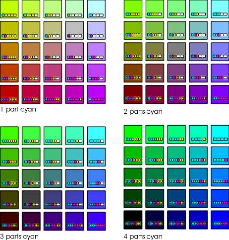
The incremental addition of cyan to this entire magenta-yellow plane will yield similar
results in the form of multiple planes of color. This third dimension of color, as in the
diagram below, is organized in terms of base color percentage (exactly as above) and each
plane is separated according to cyan content. The Color Bars once again fix the overall
volume of each color to a single value and allow us to see the actual color that each
formula represents.
|
Figure 14. Increasing Cyan content incrementally |
|
 |
|
| Applying Color Math Having completed our
derivation of an entire COLORCUBE, we revisit the color theory basics from the beginning
of the chapter and attempt to prove these operations using Color Math. In doing so we will
introduce tools and techniques that will assist our understanding of CMY addition and
subtraction as well as create a visual grounding to Color Math procedures.
Color Bars
| Horizontal bars of color were used
extensively during the construction of the COLORCUBE to graphically depict the base and
non-base content of each color they represented. They were extremely useful in allowing us
to detect and map the patterns that exist within a color space. In this section these
diagrams become accessories to the addition of color and precursors to actual Color Math. |
|
Figure 15. |
|

|
Remembering that each Color Bar is standardized to a single set length, we are able to
add these fixed amounts together in order to determine the configuration of their sum.
For example, a given quantity of 100% white plus an equal amount of 100% primary yellow
would yield a color that is half base, half non-base with a 50% yellow hue.
Figure 15 demonstrates this graphically. It shows that once the input colors are
combined and the mixture is reset to the size standard of the original Color Bar(s), the
resulting color is one that contains equal parts white base and yellow primary.
| Figure 16. |
|
The diagram to the left is another
situation that involves base white. However, this example shows the second input to be a
color containing unequal multiple primaries. When these Color Bars are added together
we can see that the sum contains four parts base white to four parts non-base primary,
which is made up of three parts magenta and one part yellow.
Once this result is subsequently resized to the standardized length, we learn that the
four white squares are proportionately equal to half of the resulting color. Likewise, the
primaries magenta and yellow occupy 1.5 and .5 of the remaining units, respectively. |

|
|
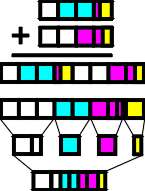
When adding colors using Color Bars, the presence of three primaries adds complexity to
the equation but the procedure for solving it is the same.
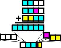
| Figure 17 shows the summarization of
three mixed colors. Each of the ingredients are gathered and grouped according their CMYW
category. After this sorting process, these input values are sized down to the normal
Color Bar in order to discover the formula of the resulting color.
Grasping the need to calibrate all color combinations to a fixed amount is important
because this normalization process allows us to estimate the colors with which we are
dealing using the cube diagrams in the previous section. Having become familiar with the
patterns inherent to the COLORCUBE, we can navigate within that color space using the
Color Bars as guides. |
|
Figure 17. |
|
|
| Figure 18. |
|
Let us take for our next equation
the sums of the last two operations and use them as inputs. After adding the Color Bars
together, we can sort and recalibrate the sum to a fixed amount with all of the
constituent elements intact. It should be clear by now that the usefulness of this
"Color Bar" addition is severely compromised by the increasing complexity of the
operations and a general inability to distinguish minute proportions with any degree of
precision. Alleviating this requires a Color Math process that relies strictly on the
objectivity of percentage values and quantities of color rather than that of a guessing
science. |
|
|
|
| Color Boxes A method that addresses our need for
exact numbers while retaining the benefits granted us by the Color Bars must begin with
the information on hand being organized in a practical manner. The tables introduced here
place the CMY formula of a color in a usable format that allows any color to be added
and/or subtracted. It also takes into consideration the volume of color as well.
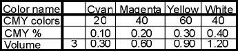
Suppose we have three units of color gold (C20 M40 Y60) which is one of our inputs in a
Color Math operation. Our first step is to determine its percentage base content by
subtracting the CMY quantity that is greatest from 100. In this instance, yellow is most
dominant with a value of 60. Consequently, this color contains 40% base white.
The remaining 60% consists of primary colors cyan, magenta and yellow in relative
proportion to the color’s CMY formula. Thus, we divide each of the primary quantities
(20, 40, and 60) by the sum of those primaries (120) and multiply each by 60%. This yields
adjusted weights of 10, 20 and 30% for CMY respectively. We find that this shade of gold
is 10% cyan, 20% magenta, 30% yellow and 40% white. The table below summarizes this
information as well as provides the volume calculation.
|
Figure 19. Table for CMY breakdown |
|
 |
The next diagram displays the above information in a graphical format that actually
maps the relative strength of each of the CMY element and places the overall proportion of
the base color in the forefront. This Color Box format adds a visual dimension to the CMY
formula and offers insight to the color itself.
|
Figure 20. Color Box |
|
 |
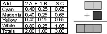
This Color Math documentation also makes use of tables and diagrams that isolate the
current operation. These are fairly self-explanatory in that they summarize the actual
quantities and volumes of color that are being added or subtracted in columnar form. In
figure 21, "A" and "B" represent the input colors and "C"
symbolizes the resultant color.
|
Figure 21. Table of operation and accompanying graphic. |
|
 |
Introduction Complete
At this point, the basics of Color Math have been fully explained. We pause here to
welcome comments from you that either accept or reject the theories explored here. Please
contact Spittin’ Image Software for more
information on Color Math and look for future developments on this fascinating subject on
this website. |
|